Validity-Preserving Hierarchical RL for Joint Routing and Switch Placement in EDA

This post presents our paper, Validity-Preserving Hierarchical RL for Joint Routing and Switch Placement in EDA (1), currently under review. It proposes a hierarchical framework for jointly optimizing switch placement and logical communication routes in Electronic Design Automation (EDA).

TL;DR: Part of designing an on-chip communication network involves placing switches (routers that redirect incoming packets toward their destination), choosing the physical connections between components, and assigning a route to each pair of communicating components. We introduce a hierarchical framework to optimize these decisions jointly using Reinforcement Learning (RL). The process starts with a single switch connecting all communicating pairs, and iteratively “zooms in” to refine the routing. At each step, it duplicates a switch, places the two copies, and locally refines the routes that traversed the original switch. After each complete cycle, every communicating pair still has exactly one assigned loop-free route. Under our simplified model, this restricted search space also contains at least one optimum, so the search does not have to spend most of its compute on designs that violate the routing constraints.

Preliminaries

Designing a chip is an extremely difficult and costly task. Automating part of the workflow can improve the solutions found and make the design process faster, allowing for more iterations. RL has already shown promising results in chip design: AlphaChip (2), for example, learns to place chip macros. Here, we focus on a different task: building the communication infrastructure between components whose positions are already fixed.

The task we are interested in is the following:

1. Most components are already placed. Some regions, called blockages, are reserved: switches cannot be placed inside them, and wires cannot cross their interiors. We are given pairs of components that communicate; those sending packets are called initiators, and those receiving them are called targets.
2. Each communicating initiator–target pair needs one assigned loop-free route. This requires placing switches and wires on the floorplan, and deciding which connections each pair uses.
3. There is an inherent trade-off: more direct connections can shorten communication routes, but increase the total amount of wire. Sharing connections saves wire, but may make individual routes longer.

The following figures show all our problem instances and their corresponding solutions found by our algorithm. Our algorithm needs to place switches (the yellow circles) and select a path for each communicating initiator–target pair. These paths are shown below each floorplan.

Pretraining floorplan 1 / 24 — best solution found by Gumbel MCTS.

Pretraining floorplan 2 / 24 — best solution found by Gumbel MCTS.

Pretraining floorplan 3 / 24 — best solution found by Gumbel MCTS.

Pretraining floorplan 4 / 24 — best solution found by Gumbel MCTS.

Pretraining floorplan 5 / 24 — best solution found by Gumbel MCTS.

Pretraining floorplan 6 / 24 — best solution found by Gumbel MCTS.

Pretraining floorplan 7 / 24 — best solution found by Gumbel MCTS.

Pretraining floorplan 8 / 24 — best solution found by Gumbel MCTS.

Pretraining floorplan 9 / 24 — best solution found by Gumbel MCTS.

Pretraining floorplan 10 / 24 — best solution found by Gumbel MCTS.

Pretraining floorplan 11 / 24 — best solution found by Gumbel MCTS.

Pretraining floorplan 12 / 24 — best solution found by Gumbel MCTS.

Pretraining floorplan 13 / 24 — best solution found by Gumbel MCTS.

Pretraining floorplan 14 / 24 — best solution found by Gumbel MCTS.

Pretraining floorplan 15 / 24 — best solution found by Gumbel MCTS.

Pretraining floorplan 16 / 24 — best solution found by Gumbel MCTS.

Pretraining floorplan 17 / 24 — best solution found by Gumbel MCTS.

Pretraining floorplan 18 / 24 — best solution found by Gumbel MCTS.

Pretraining floorplan 19 / 24 — best solution found by Gumbel MCTS.

Pretraining floorplan 20 / 24 — best solution found by Gumbel MCTS.

Pretraining floorplan 21 / 24 — best solution found by Gumbel MCTS.

Pretraining floorplan 22 / 24 — best solution found by Gumbel MCTS.

Pretraining floorplan 23 / 24 — best solution found by Gumbel MCTS.

Pretraining floorplan 24 / 24 — best solution found by Gumbel MCTS.

Fine-tuning floorplan 1 / 4 — best solution found by fine-tuning pretrained Gumbel MCTS.

Fine-tuning floorplan 2 / 4 — best solution found by fine-tuning pretrained Gumbel MCTS.

Fine-tuning floorplan 3 / 4 — best solution found by fine-tuning pretrained Gumbel MCTS.

Fine-tuning floorplan 4 / 4 — best solution found by fine-tuning pretrained Gumbel MCTS.

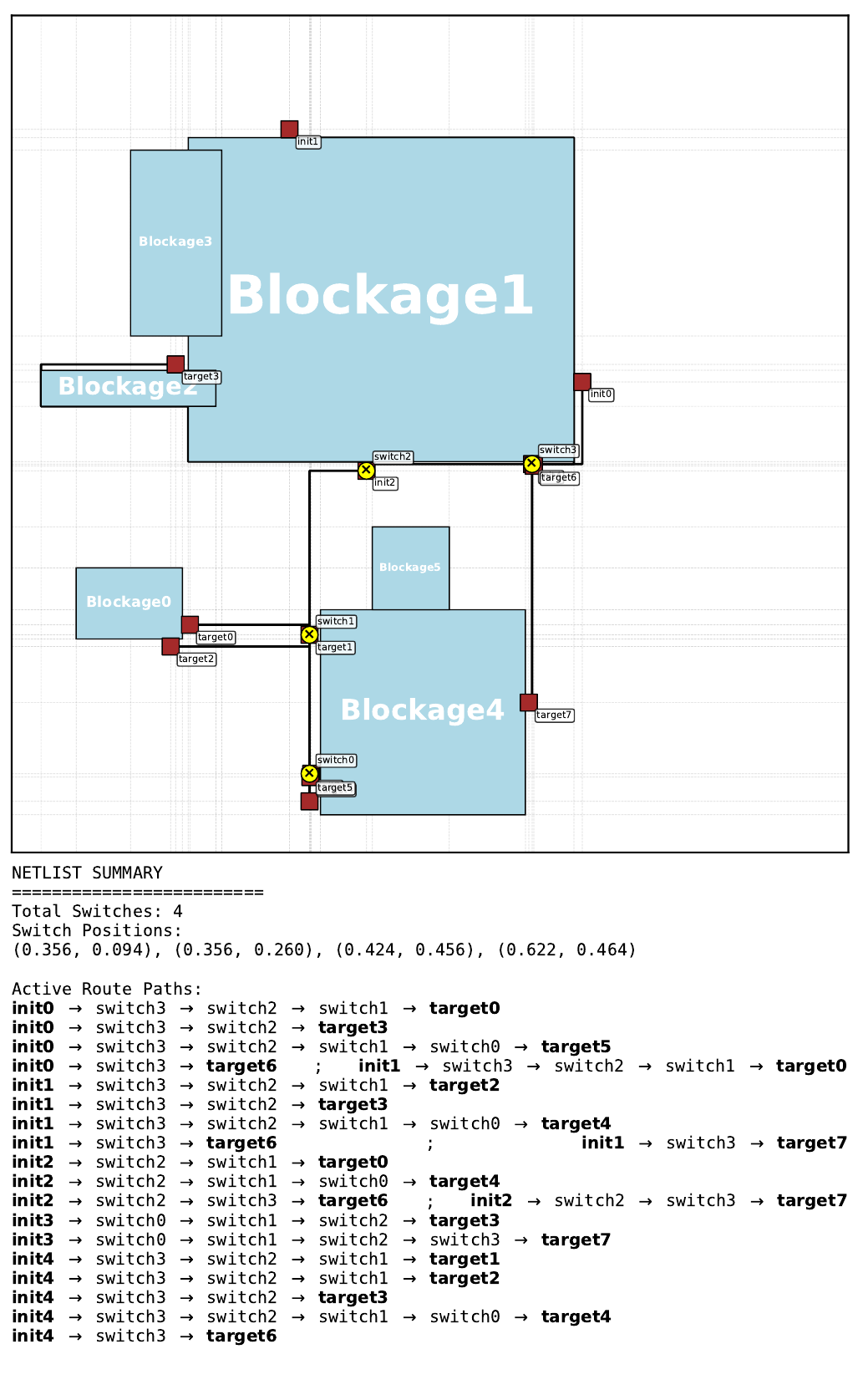
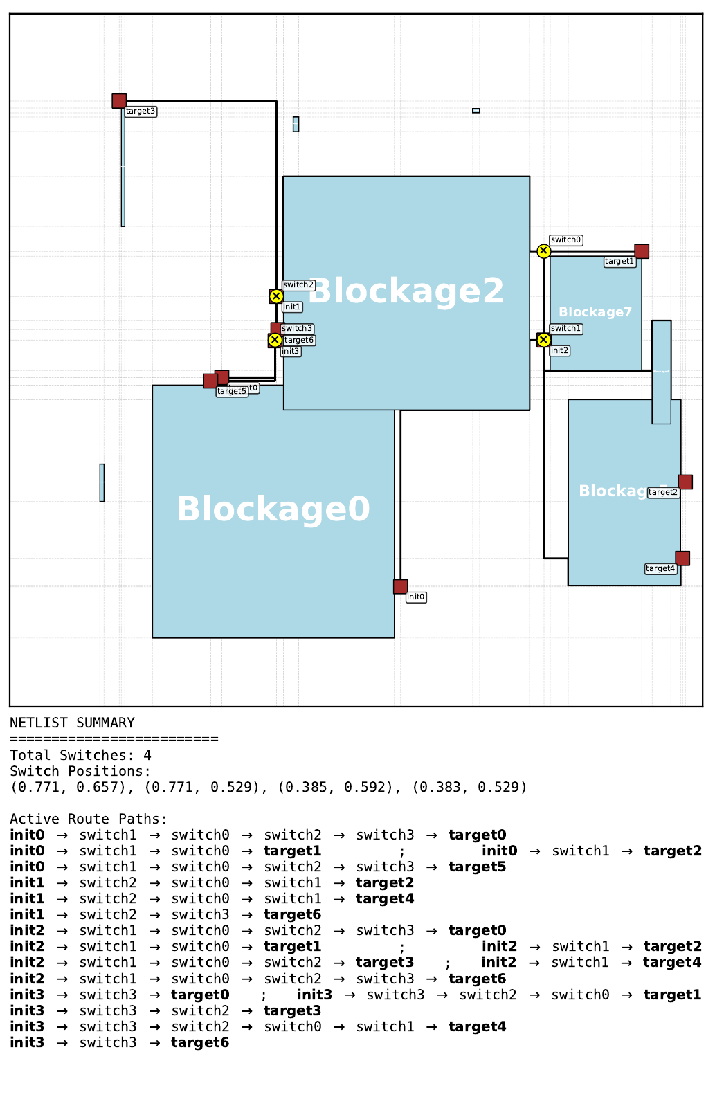
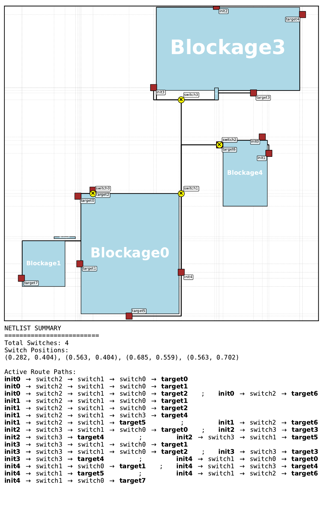
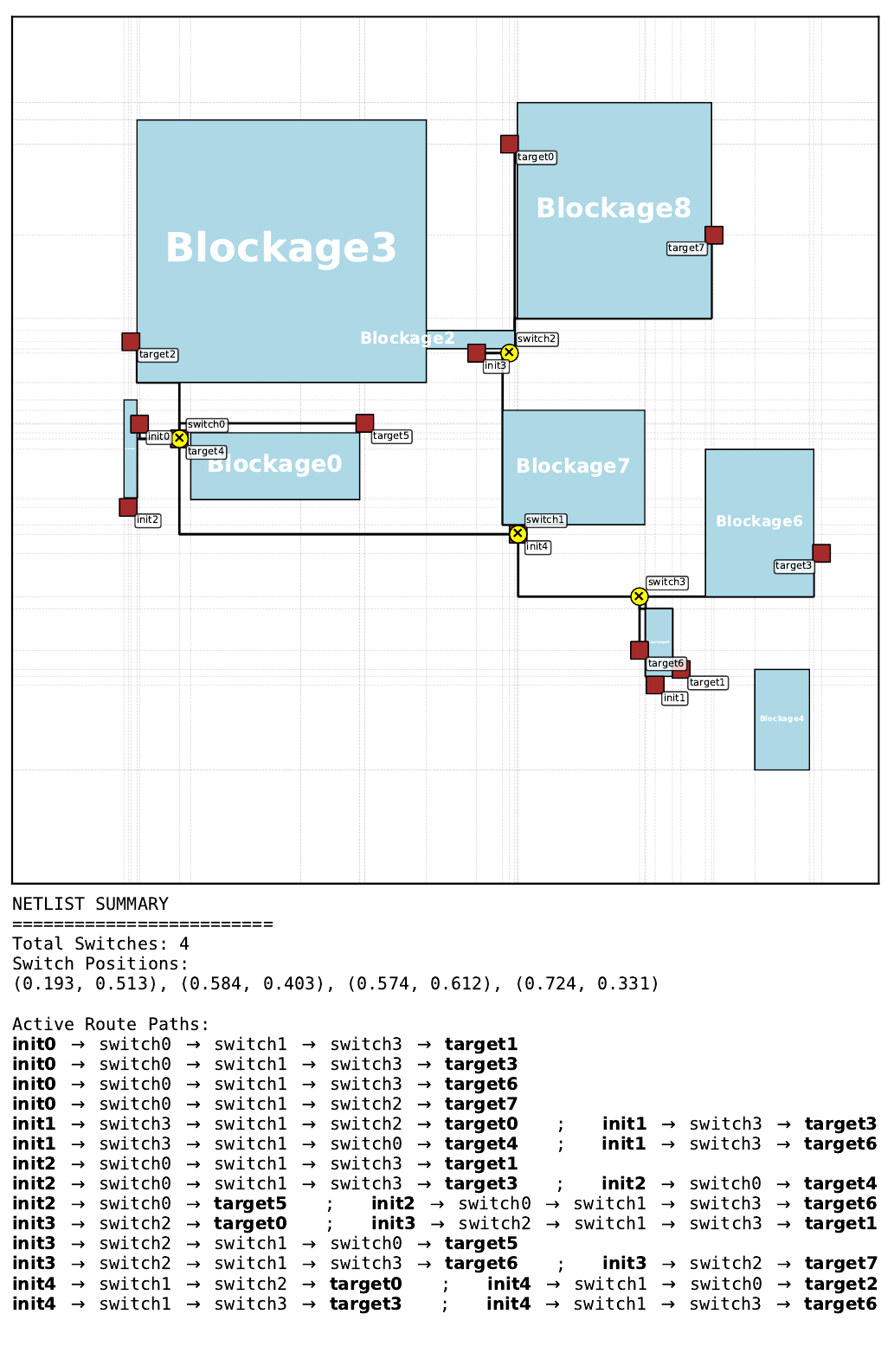
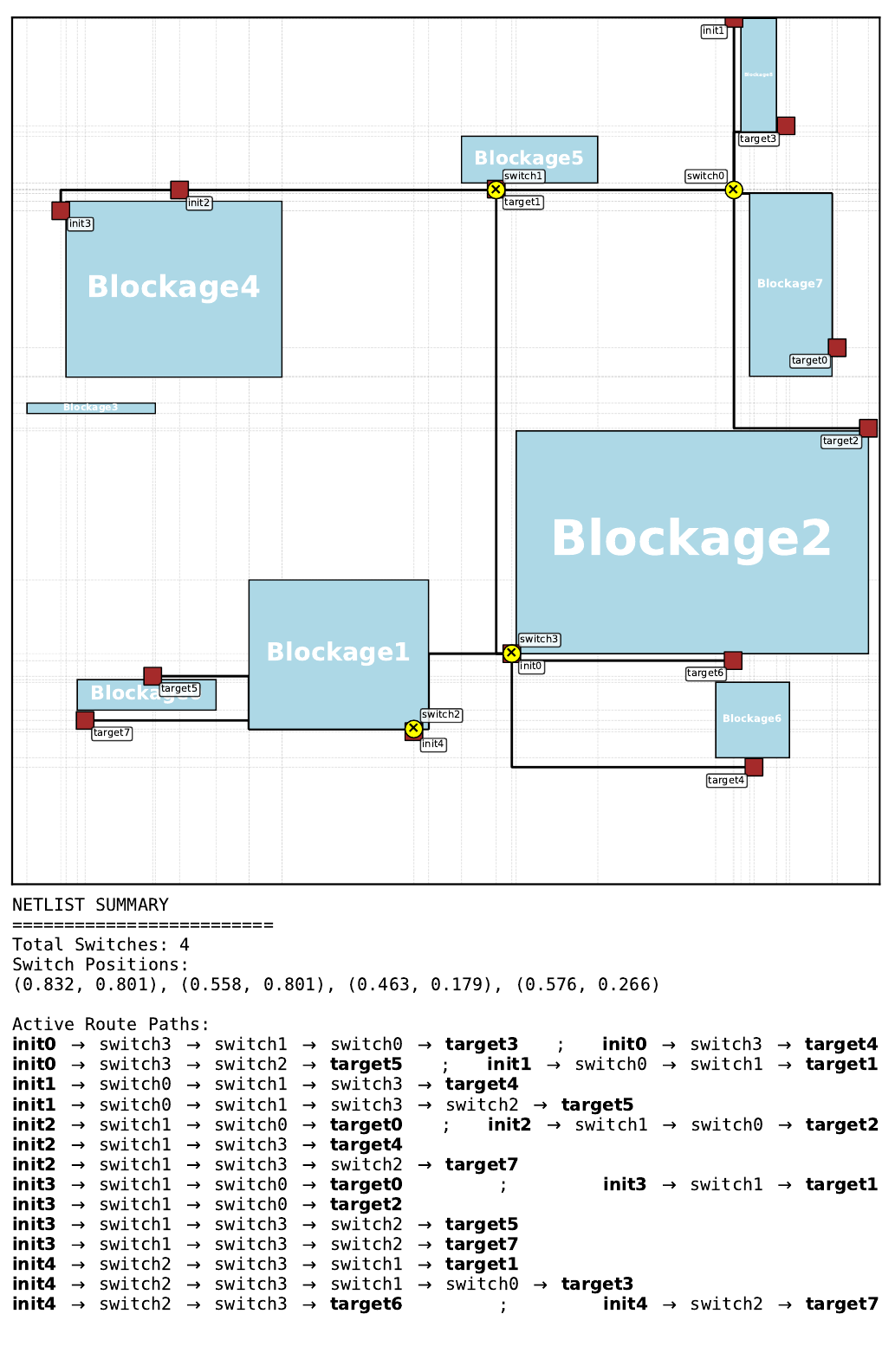
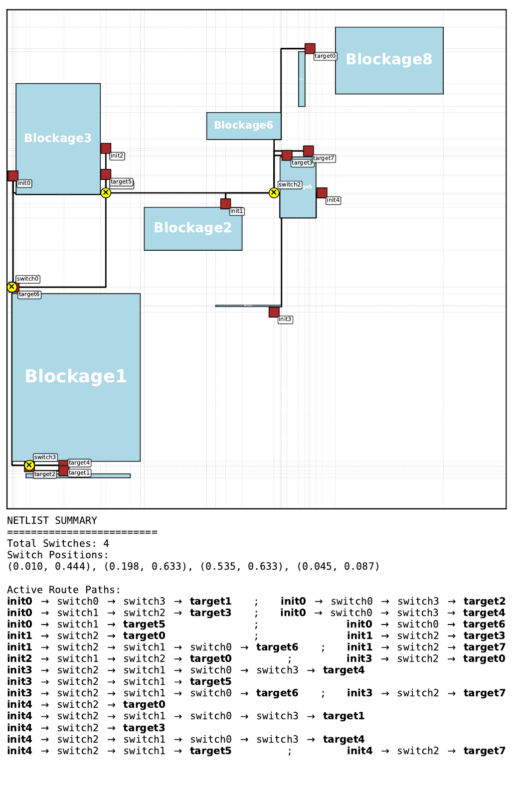
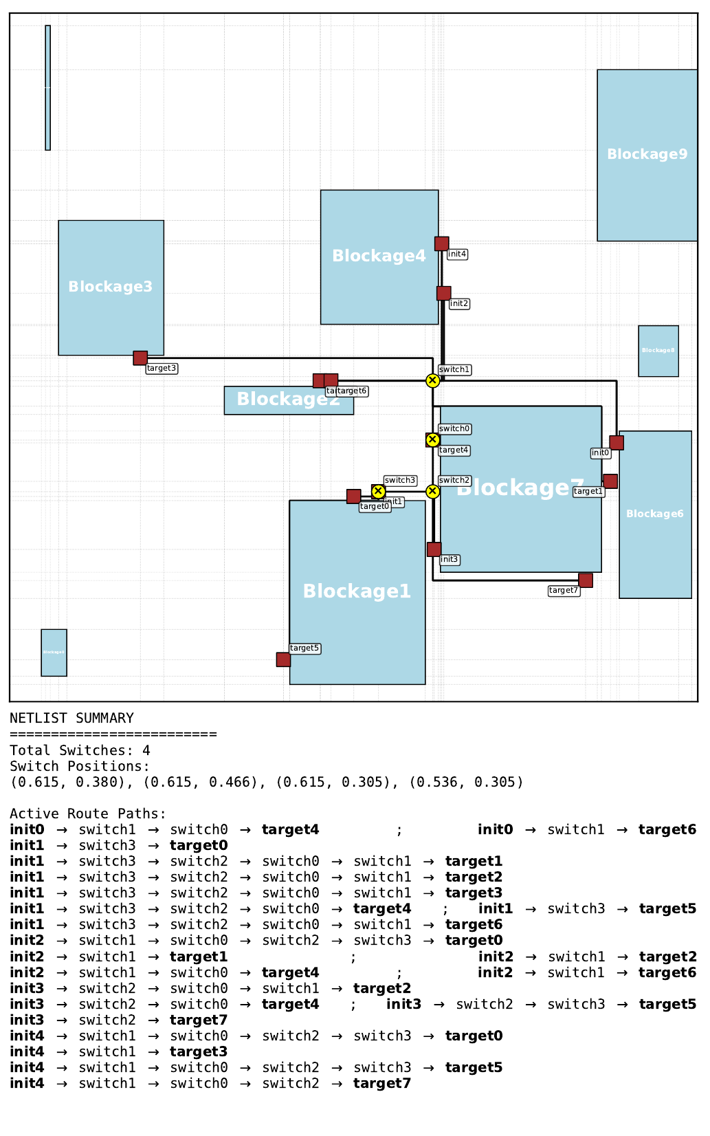
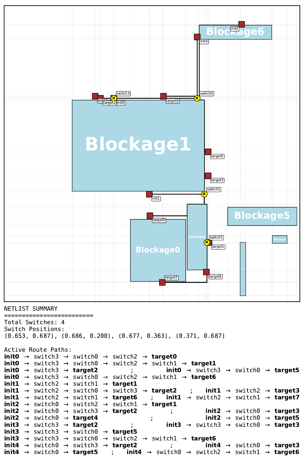
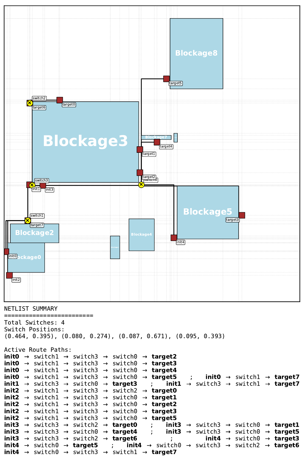
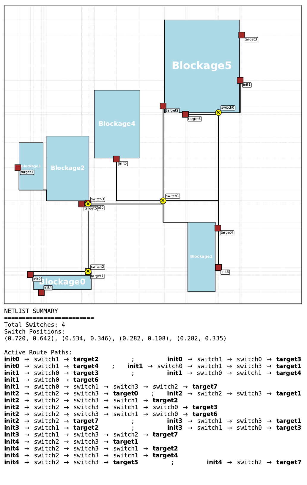
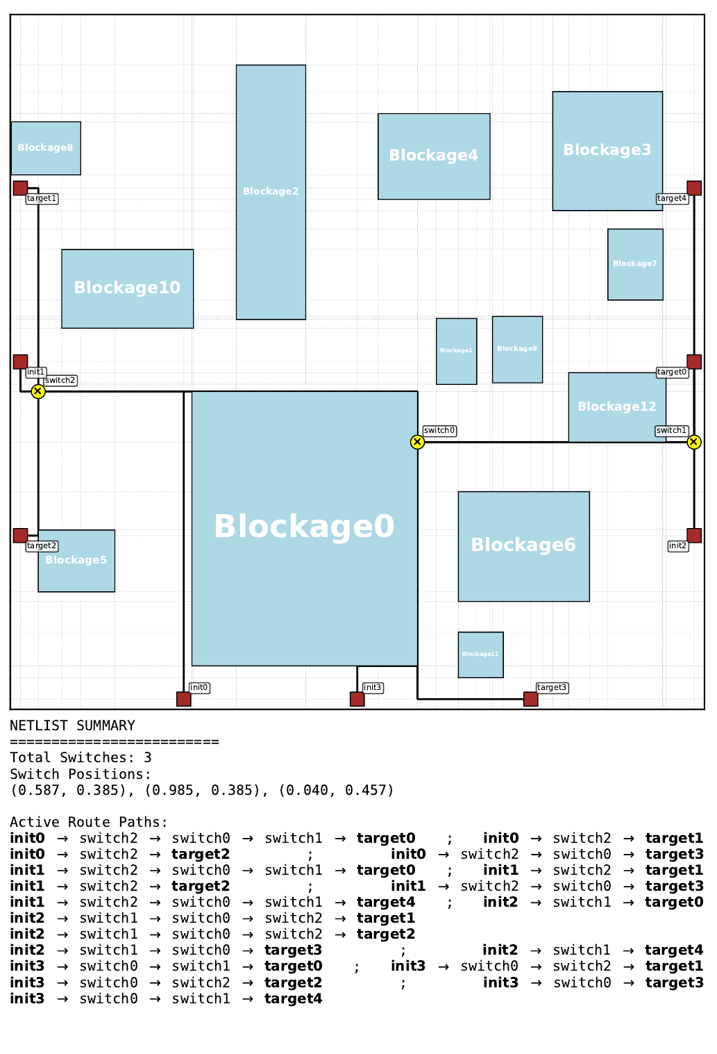
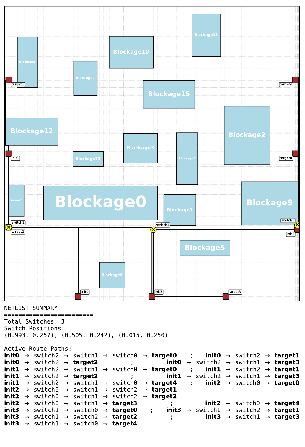
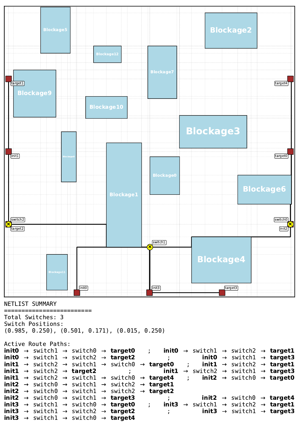
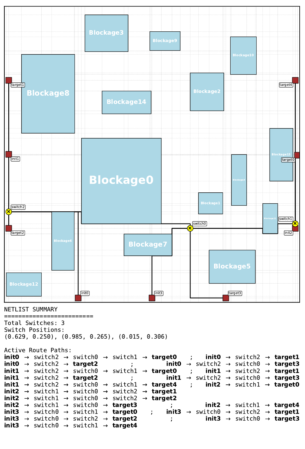
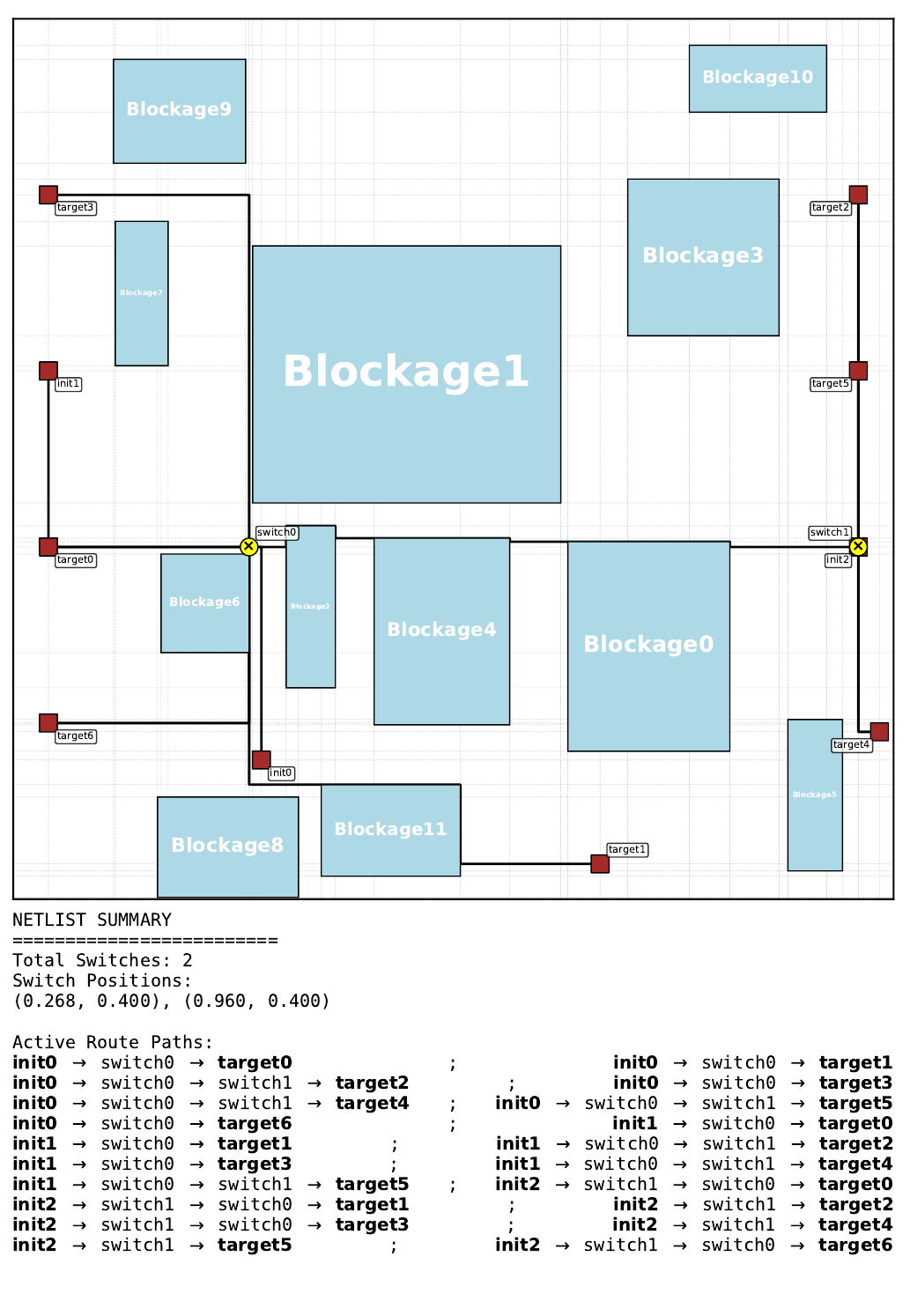
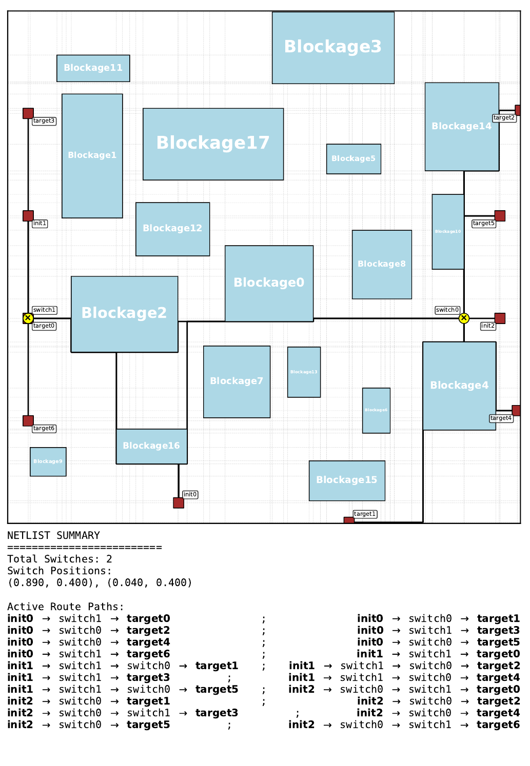
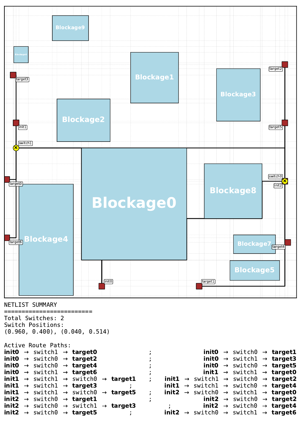
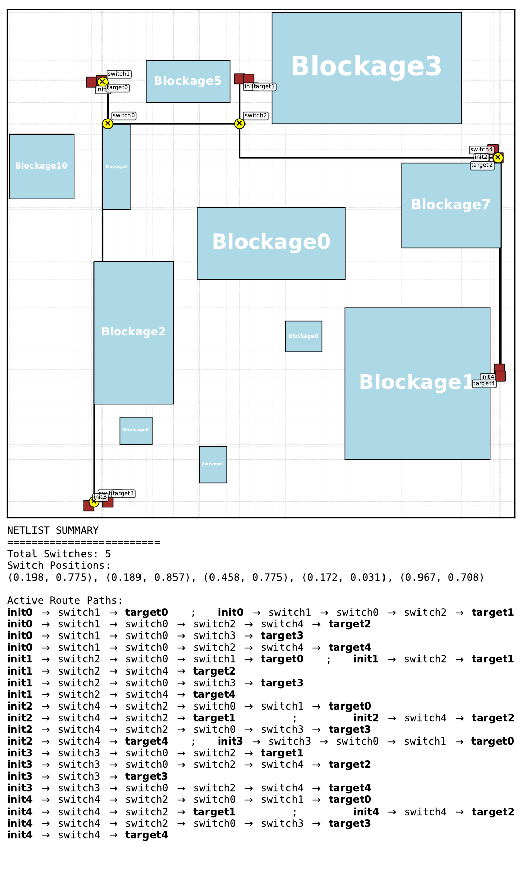
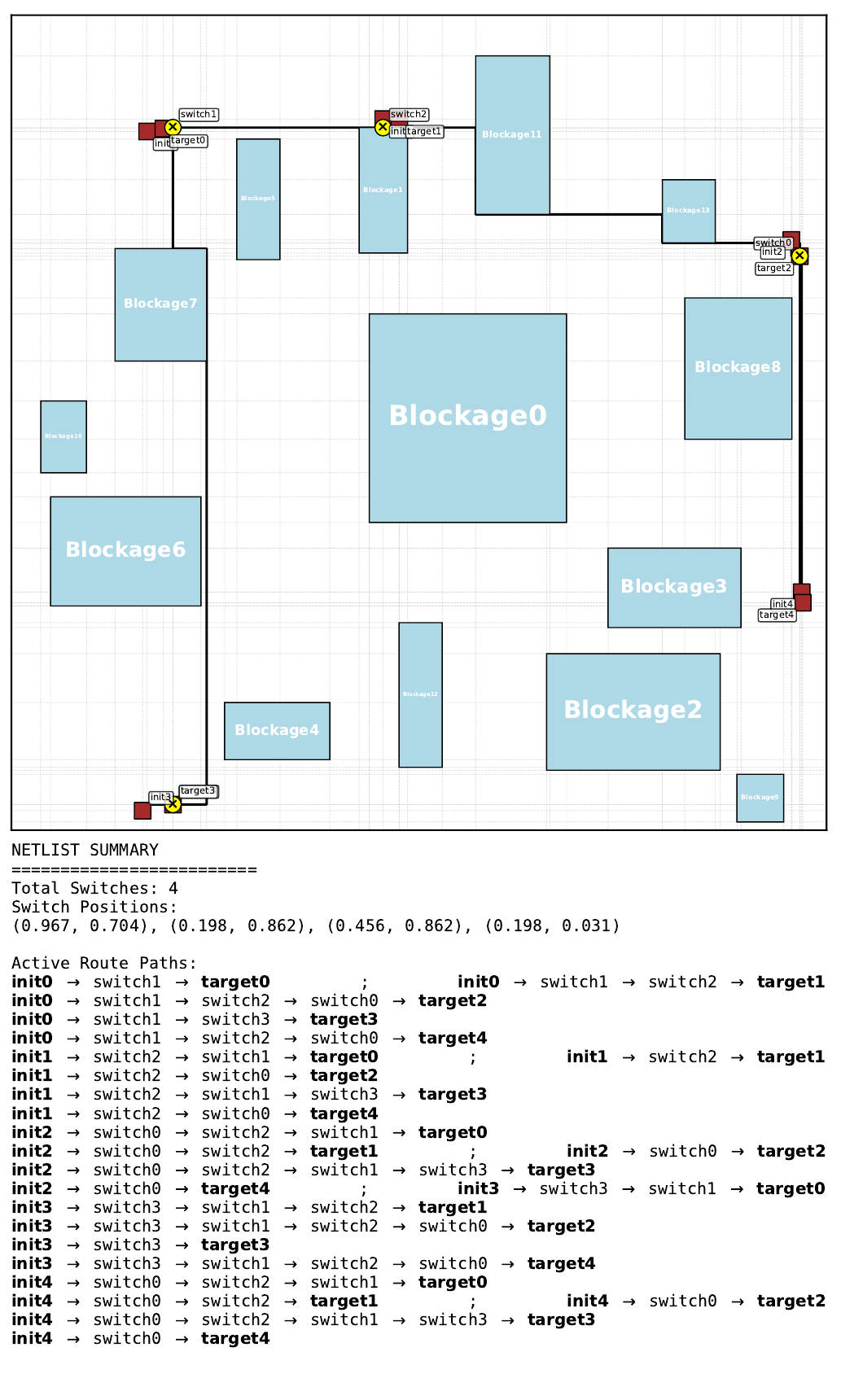
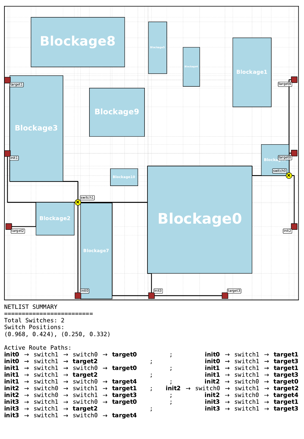
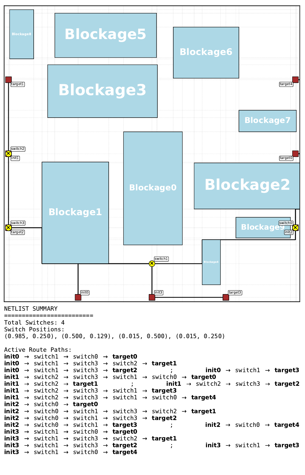
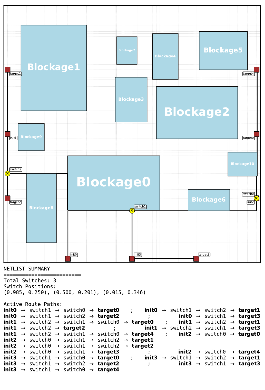
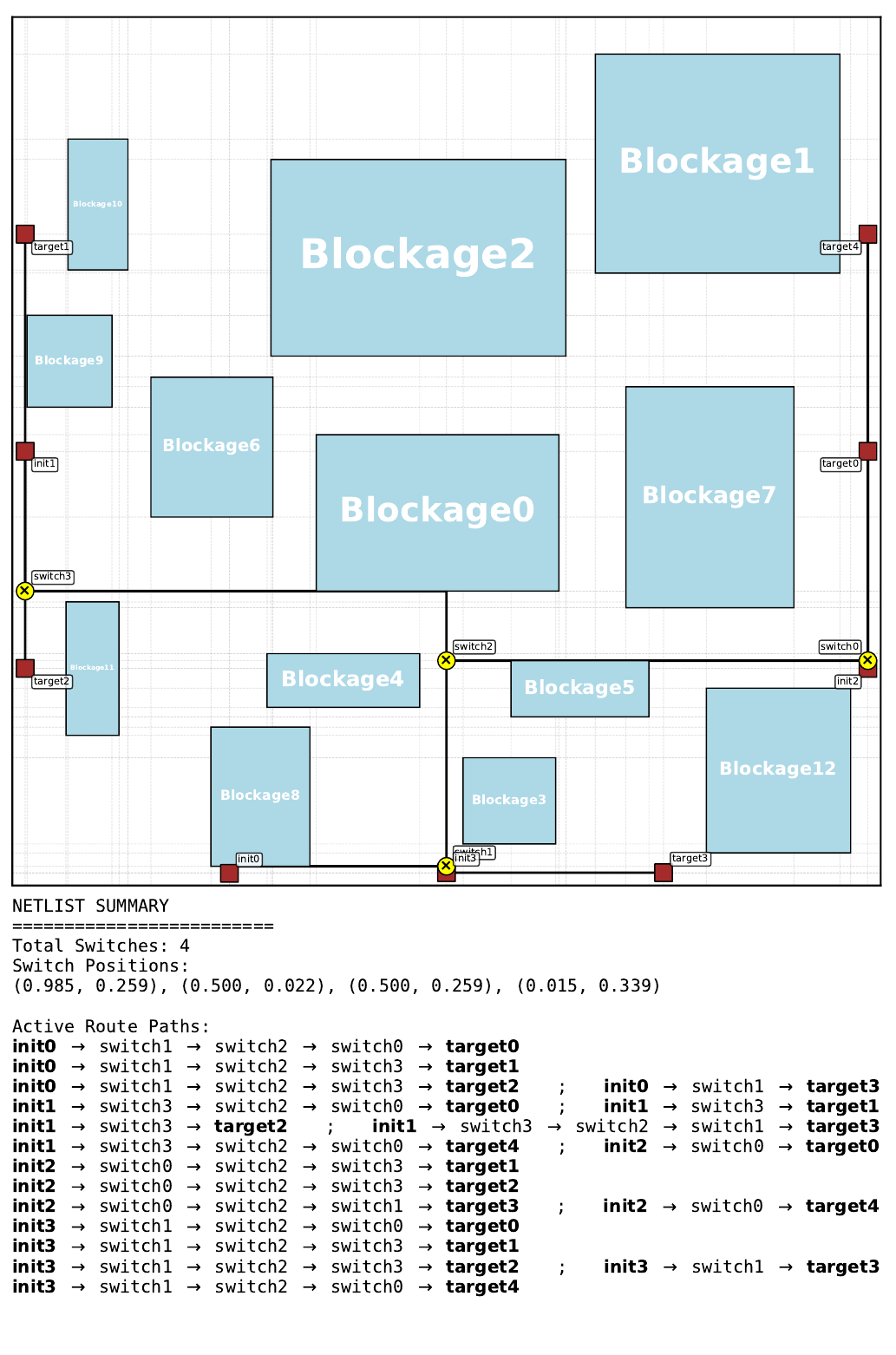
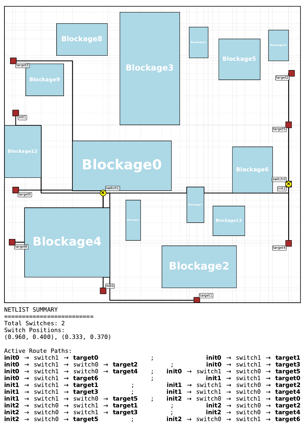
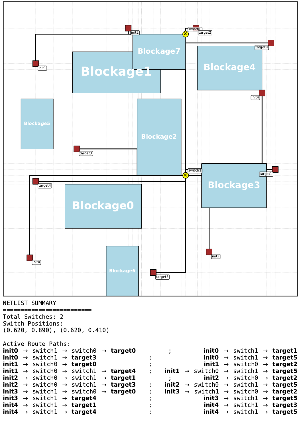
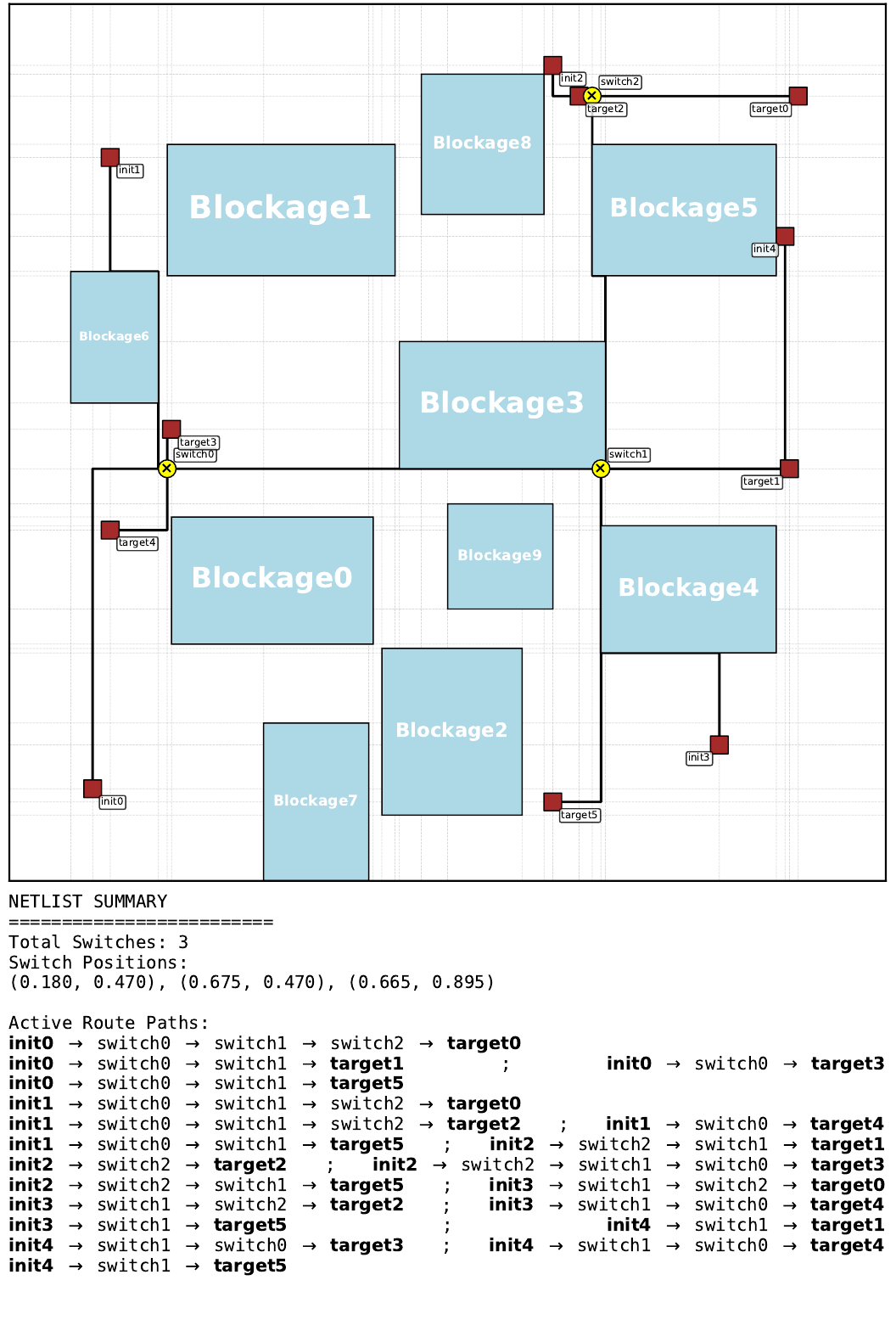
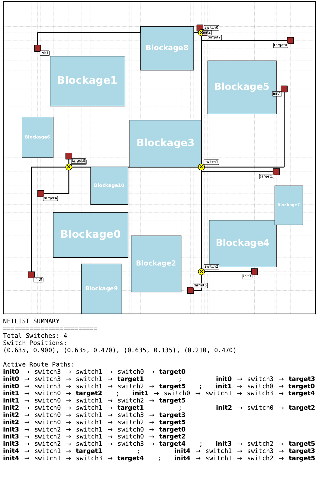
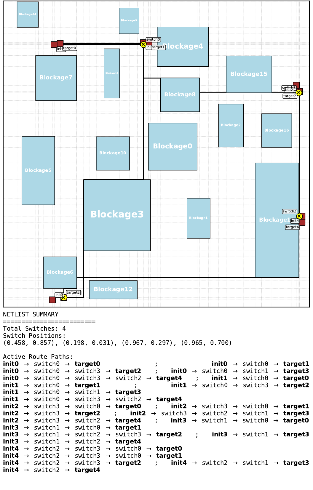
Our objective is to find an efficient and scalable method for jointly placing switches and selecting these routes. As a first step, we use a deliberately simplified model: we only optimize wirelength and communication-route length, rather than directly modeling latency. We also neglect component dimensions and pin-level requirements, and do not model congestion, bandwidth, routing layers, or vias.

Problem Formulation

Setting

Let $\mathcal I$ and $\mathcal T$ be the sets of initiators and targets, with fixed positions on a rectangular floorplan $\Omega$. The required communications are given by $\mathcal R\subseteq\mathcal I\times\mathcal T$, and the rectangular blockages by $\mathcal B$.

A solution has two components:

• Placement: choose a set of switches $\mathcal S$, with at most $S_{\max}$ switches, and place them outside blockage interiors.
• Routing: for every pair $(i,t)\in\mathcal R$, choose a loop-free directed path $\pi_{i,t}$ from $i$ to $t$. Each path must traverse at least one switch, and all its intermediate nodes must be switches.

Together, these paths define the routing graph: its edges are exactly the connections used by at least one communication route. The graph itself does not have to be a tree; the loop-free constraint only applies to logical routes.

We consider rectilinear wires, made only of horizontal and vertical segments. For two connected nodes $u$ and $v$, we denote the length of a shortest rectilinear connection avoiding blockage interiors by $d_{\mathcal B}(u,v)$. Without an obstacle-induced detour, this is simply the Manhattan distance \(d_{\mathcal B}(u,v)=\lvert x_u-x_v\rvert+\lvert y_u-y_v\rvert\).

Combinatorial Problem Formulation

Denote the edge set of the routing graph by $\mathcal E$, we distinguish:

• \(L_{\mathrm{wire}} = \sum_{\{u,v\}:\,(u,v)\in\mathcal E\,\lor\,(v,u)\in\mathcal E} d_{\mathcal B}(u,v)\): the total length of the physical wire connections. A shared connection is counted once, regardless of how many pairs use it or in which direction.
• \(L_{\mathrm{route}} = \sum_{(i,t)\in\mathcal R}\sum_{(u,v)\in E(\pi_{i,t})} d_{\mathcal B}(u,v)\): the sum of the lengths of all assigned communication routes. Here, a connection is counted each time a route uses it. This is used as a proxy for latency.

The goal is to find a feasible placement and routing that minimizes $ L_{\mathrm{wire}}+\lambda L_{\mathrm{route}}, $ subject to the switch budget and the routing constraints above. In our experiments, we use $\lambda=\tfrac12$.

Our Method

Route Nodes

(a) Routing graph with communication pairs stored as edge attributes.

(b) Graph after conversion to route nodes. Nodes labeled (1) correspond to pair (1, 1), and those labeled (2) to pair (2, 2).

Route-node conversion: each communication pair traversing an edge is represented explicitly by a route node.

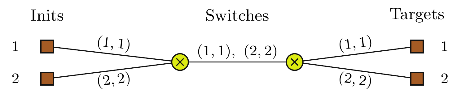
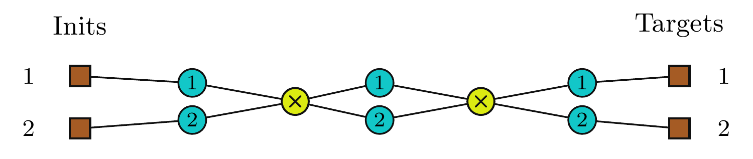
Directly manipulating the initiator–target pairs allowed to traverse a wire is tedious. Instead, we represent those attributes as explicit route nodes in the graph. Each connection is replaced by one intermediate route node for every communication pair that uses it, as shown above. This is more convenient for us: allowing or forbidding a pair to use a connection becomes a matter of connecting or disconnecting its route node. Assigning paths then reduces to filtering edges in the route graph.

Extended Hanan Grid

The extended Hanan grid, including coordinates from blockage corners.

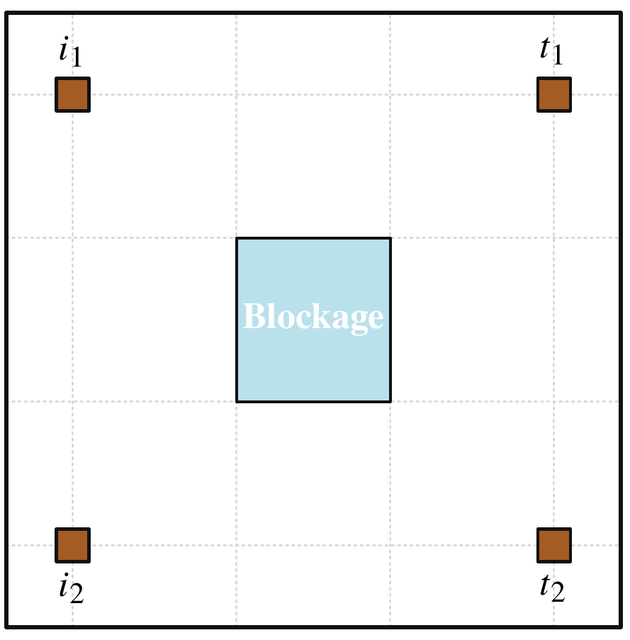
The Hanan grid consists of the horizontal and vertical lines passing through initiators and targets (3). Since our floorplans also contain blockages, we add lines passing through their corners. Switches can be placed at grid intersections outside blockage interiors. For the rectilinear model studied here, we show that there exists an optimal solution with all switches on this extended grid. We can therefore replace continuous placement decisions with a finite set of candidate positions without excluding every optimum.

Expansion–Refinement

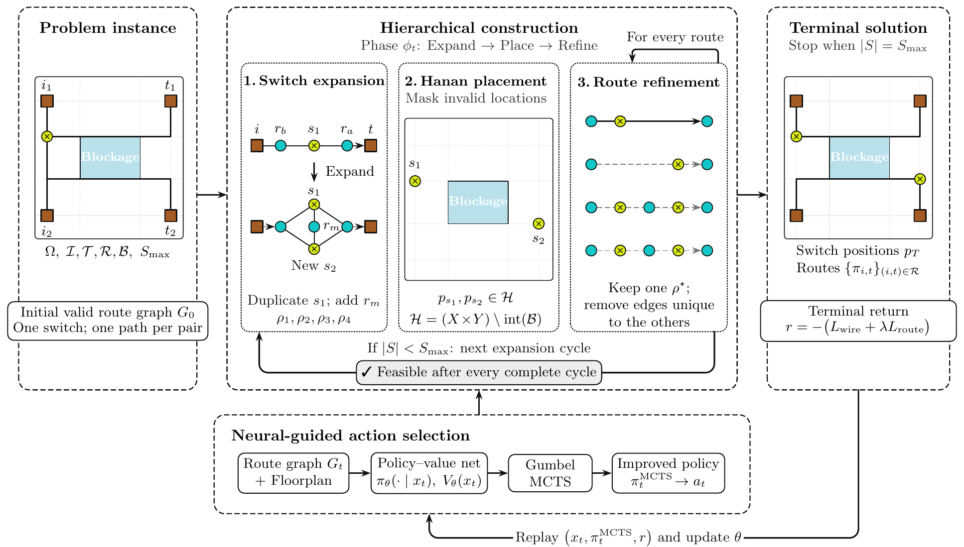
Our method operates directly on the graph with route nodes. It starts with a single switch connecting every required initiator–target pair, and gradually constructs the solution through three steps:

1. Switch expansion: select a switch and duplicate it at the same position, copying its connectivity. For each route traversing the original switch, introduce an additional route node between the two switches.
2. Switch placement: place both the original switch and its new copy on intersections of the extended Hanan grid.
3. Route refinement: for each affected communication pair, choose one of four local routing alternatives. Denoting the switches by $s_1$ and $s_2$, the four possibilities are: entering $s_1$ and exiting; entering $s_1$, going to $s_2$, then exiting; and the two symmetric possibilities where $s_1$ and $s_2$ are swapped.

These steps repeat until the switch budget is exhausted. This framework is attractive because it restricts the search to a subset of feasible solutions while retaining at least one optimum of our problem. Indeed, after every complete expansion–placement–refinement cycle, the solution is feasible: every communicating pair has exactly one assigned loop-free route.

PPO-EWMA and Gumbel MCTS

Now that we have defined how to construct a floorplan, we can use a search algorithm to explore the space of solutions. Our two main search algorithms come from the RL literature: a model assigns probabilities to actions, and sampled action sequences are used to update these probabilities in order to make sequences that lead to good solutions more likely. More precisely, PPO-EWMA and Gumbel MCTS start with almost uniform probabilities over the available actions and alternate between a collection phase and an update phase.

During the collection phase, sequences of actions are sampled according to the probabilities produced by the model. At the end of each trajectory, the objective value obtained for the floorplan is computed. During the update phase, the probabilities of the chosen actions are increased if they lead to a better outcome than the average result, and decreased if they lead to a worse outcome. This corresponds to PPO-EWMA.

Gumbel MCTS additionally simulates future outcomes before choosing an action. At each step of a trajectory, it runs a fixed number of simulations (800 in our case) to estimate the outcomes of various possible action sequences and uses these estimates to improve the initial probabilities before sampling an action. This improves the quality of the generated data and helps avoid diluting the model with bad actions or getting stuck in local minima, to which PPO-EWMA is very sensitive. This makes Gumbel MCTS particularly well suited to combinatorial problems.

The process can be thought of as a form of annealing: initially, actions are chosen at random, and their selection gradually becomes deterministic and concentrated on good sequences of actions.

The full pipeline is shown below. Our main algorithm for finding a good sequence of actions is Gumbel MCTS.

Experiments

Baselines

We compare: Random search (4), which selects actions uniformly at random; Genetic algorithm (5), where action sequences are evolved through mutation and crossover; PPO-EWMA (6), which learns an action-selection policy without tree search; and Gumbel MCTS (7), which combines a learned policy and value function with tree search. We also compare these methods with a Steiner-inspired heuristic, which builds the solution greedily on the extended Hanan grid using the marginal contribution of candidate actions to the objective.

Pretraining

We compare the five methods on 24 floorplans. Each optimization method gets a 48-hour budget, and the deterministic heuristic is run once. For both PPO-EWMA and Gumbel MCTS, a policy is trained jointly across all 24 floorplans. The table below reports the best objective found by each method, with lengths normalized by the side length of the corresponding square floorplan.

Gumbel MCTS finds the best objective on all 24 floorplans, with an especially visible gap on floorplans 18 and 19. The corresponding solutions can be found in the opening slideshow.

Fine-tuning

Once the policy has finished training on all 24 floorplans, we use it as an initialization on four held-out floorplans. We compare fine-tuning this pretrained policy with training from scratch, both in terms of solution quality and convergence speed. Both are trained for 24 hours.

(a) Fine-tuning floorplan 1.

(b) Fine-tuning floorplan 2.

(c) Fine-tuning floorplan 3.

(d) Fine-tuning floorplan 4.

Fine-tuning experiments on four unseen floorplans. Blue lines correspond to Gumbel MCTS, and orange ones to PPO-EWMA; solid lines correspond to pretrained initialization, and dashed lines correspond to training from scratch.

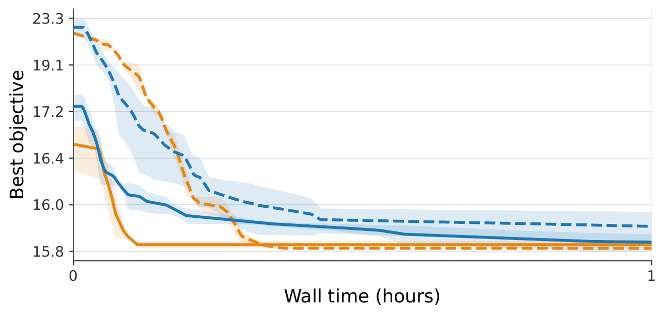
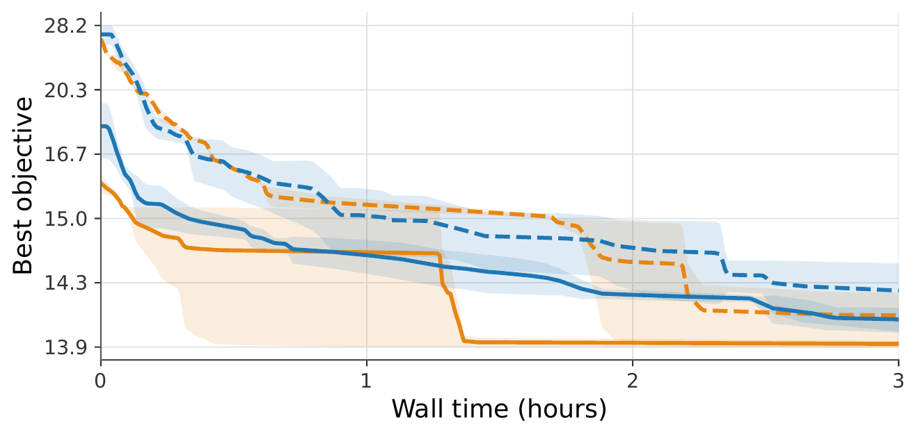
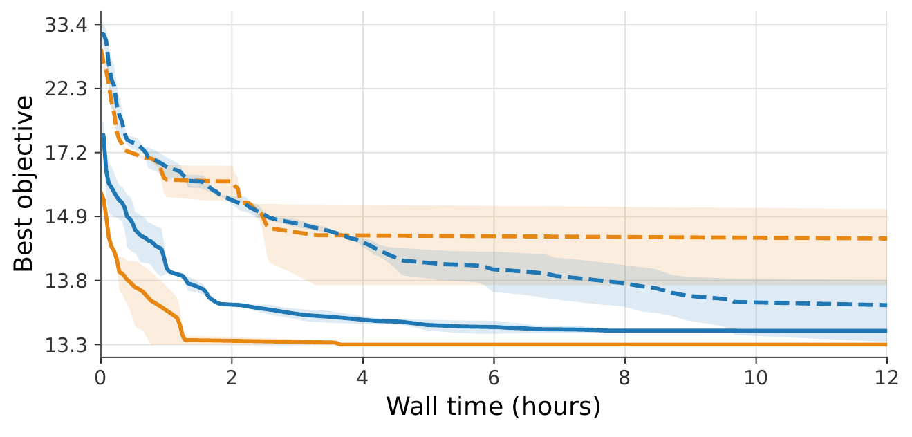
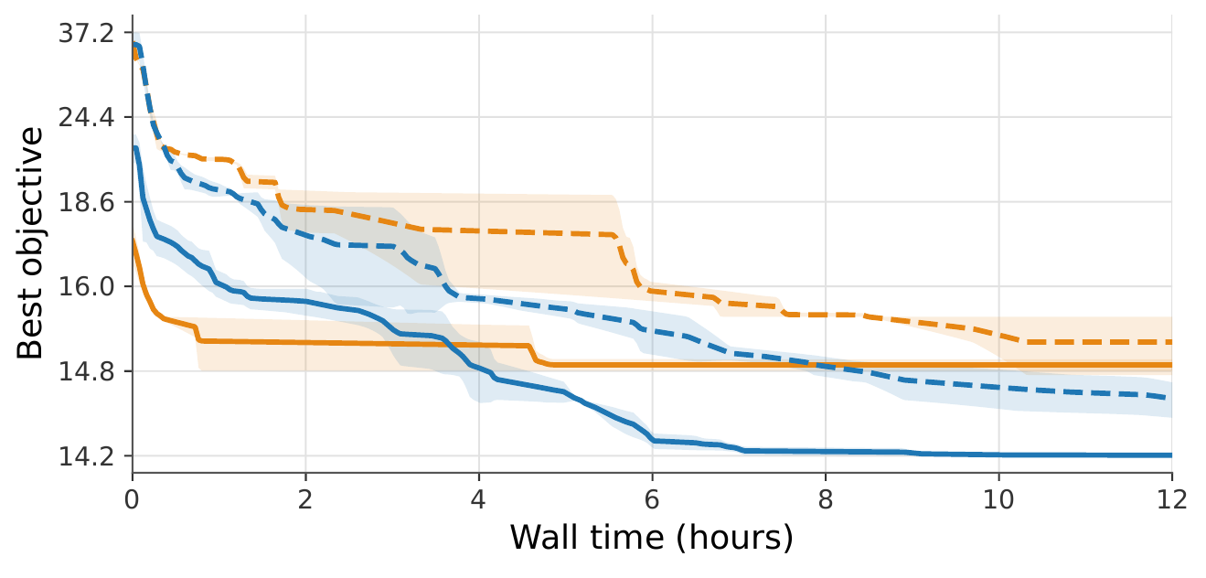
Pretraining shortcuts optimization on unseen floorplans: fine-tuning reaches competitive solutions faster than training from scratch and, on some floorplans, also finds better solutions within the available budget.

Limitations

Our experiments are limited to small-scale floorplans, and the physical model is very simplified. In particular, we neglect component dimensions and pin-level requirements, and do not model congestion, bandwidth, routing layers, or vias. Finally, route length is only a simplified geometric proxy for latency, not a detailed model.

Conclusion

This work is a first step toward scalable, automated joint routing and switch placement. Our next objectives are to make the model more realistic by integrating richer physical constraints and cost models, and to scale the method toward industrial problems.

When using our work, please cite our paper:

@misc{gailhard2026routing,
  title={Validity-Preserving Hierarchical RL for Joint Routing and Switch Placement in EDA},
  author={Gailhard, Dorian and Lecerf, Ugo and Tartaglione, Enzo and Conte, Donatello and Naviner, Lirida and Giraldo, Jhony H.},
  year={2026},
  eprint={2609.39749},
  archivePrefix={arXiv},
  primaryClass={cs.LG},
  url={https://arxiv.org/abs/2609.39749}
}

Acknowledgments

We acknowledge the ANR – FRANCE (French National Research Agency) for its financial support of the System On Chip Design leveraging Artificial Intelligence (SODA) project under grant ANR-23-IAS3-0004. This project has also been partially funded by the Hi!PARIS Center on Data Analytics and Artificial Intelligence.